How To Make an Attendance Sheet in Excel - Novice-friendly Guide

Want to learn how to make an attendance sheet in Excel for school or work purposes?

If you’re looking to upgrade your attendance tracking process, Microsoft Excel is a great choice. It allows you to store spreadsheets offline and online.

Below, I’ve explained methods to create a tracking sheet using manual, script, and template-based approaches. You can pick the one that suits you the most!

How To Make an Attendance Sheet in Excel Manually

Follow these steps in the order they appear in:

Create the Necessary Columns and Rows and Enter the Data

1. Create a blank Excel workbook where you’ll record attendance data.
2. Populate the following column headers in the order they appear here:
   • Employee ID
   • Name
   • Clock-In Time
   • Clock-Out Time
   • Total Worked Hours
   • Standard Hours
   • Overtime
   • Work Status.
3. For now, just enter the data for the Employee ID and the Name columns.

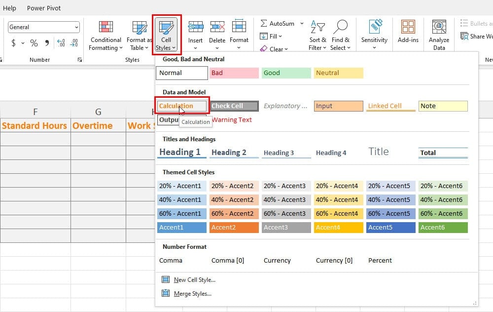
4. Now, select the dataset only with the required rows and columns.
5. Go to the Styles command block in the Home tab.
6. Click on the Cell Styles drop-down arrow and choose a style from the list.

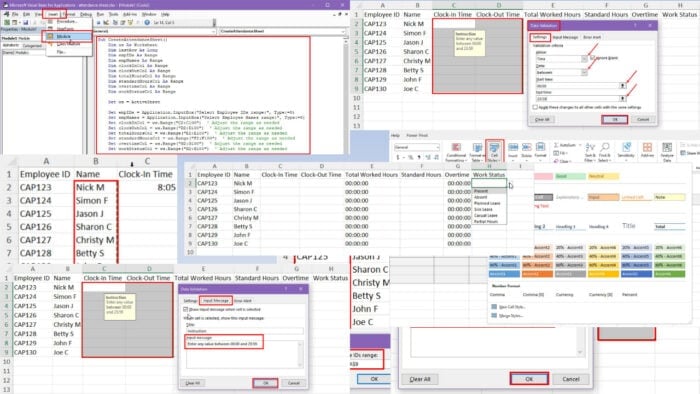
Implement Data Validation Rules

In this step, you’ll use the Excel Data Validation tool to restrict the type of content that you can add to the attendance sheet. Here’s how:

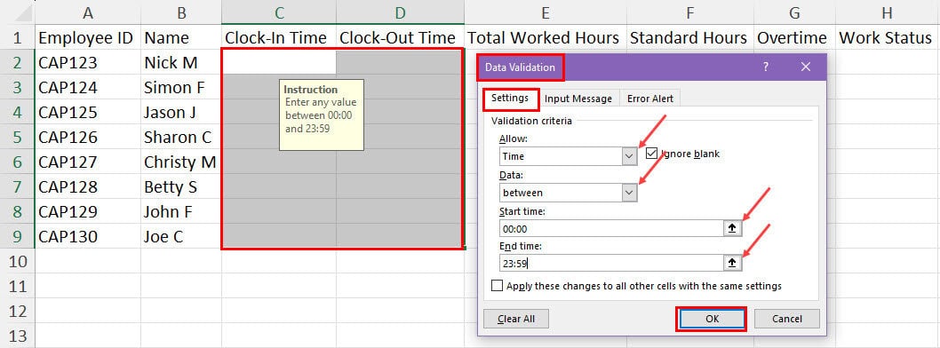
1. Select the Clock-In Time and Clock-Out Time columns with as many rows as you need.
2. Go to the Data tab and select the Data Validation rule button.
3. In the Settings tab, enter the following values in their respective fields:
   • Allow: Time
   • Data: Between
   • Start time: 00:00
   • End time: 23:59

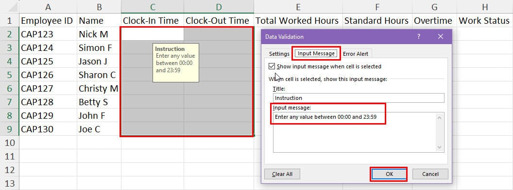
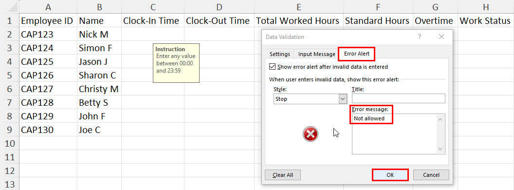
4. In the Input message field of the Input Message tab insert a text to guide users on how to enter data.

5. Enter a text in the Error Alert tab’s Error message field to show a warning if someone enters invalid data.
6. Click OK to apply the changes you’ve made.

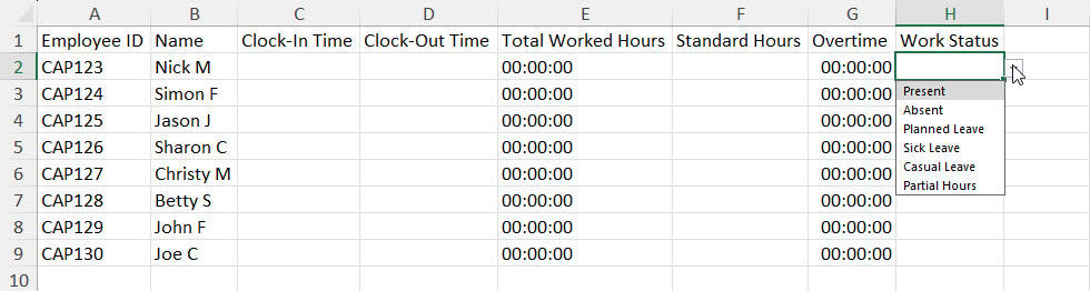
7. Now, select the Work Status column.
8. Bring up the same Data Validation tool.
9. Choose List in the Allow drop-down menu in the Settings tab.
10. Type in the following text strings:

Present, Absent, Planned Leave, Sick Leave, Casual Leave, Partial Hours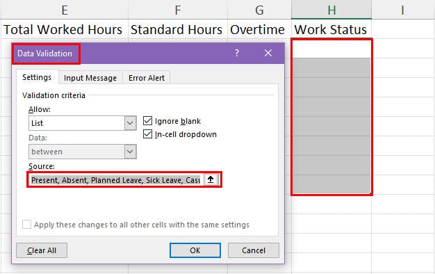

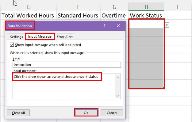
11. Go to the Input Message tab and enter instructions so the employees or students know what to type in this field.
12. Click OK to enforce the Data Validation rules.

At this stage, you’ll also need to enter the minimum working hours required for a full workday in the Standard Hours column.

To accomplish this, select the entire column below the header and select the Time formatting from the Number drop-down menu of the Home tab.

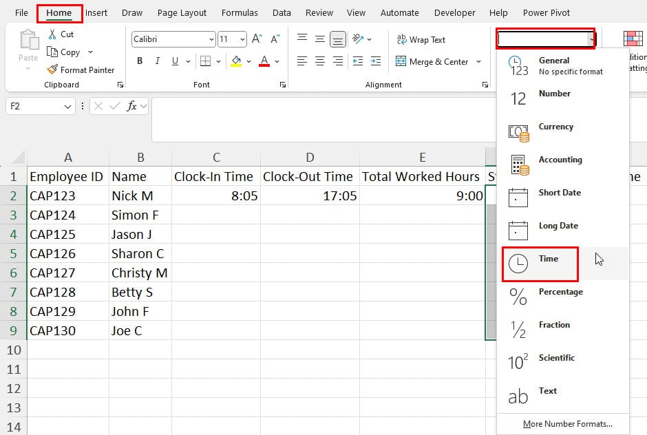
You can now enter the workday hours, like 08:00 in one cell, and copy the value in all the rows below the column.

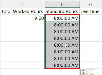
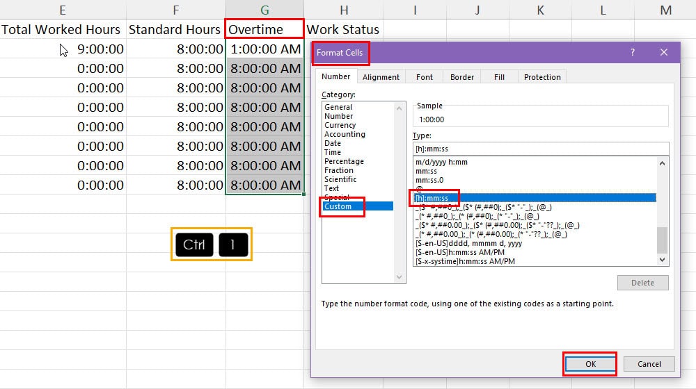
Select all cells except the column header again, press Ctrl + 1, and select the [h]:mm:ss custom number formatting code. Click OK to apply the formatting style.

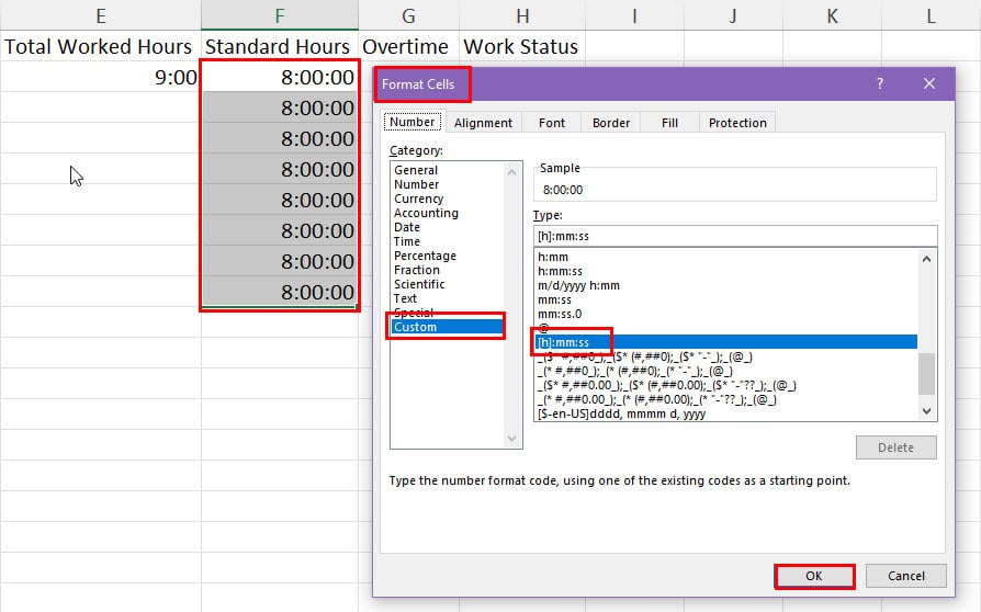
This will transform the 08:00:00 AM format of working hour value to a 8:00:00 format.

Enter Formulas To Calculate Totals

Now, you’ll learn which formulas to use and the syntaxes to automatically calculate working hours, overtime, etc.

1. In the first cell below the Total Worked Hours enter the following formula to calculate the working hour:

=D2-C2

2. Use the fill handle from the first cell to drag down to copy the same formula to the rest.
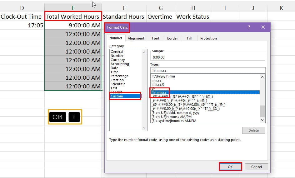
3. You should see the calculated time entries as 9:00:00 AM, 12:00:00 AM, etc.
4. Select the cell values below the column header, press Ctrl + 1, and choose the [h]:mm:ss formatting code in the Custom Category menu.
5. Click OK to apply the formatting style.

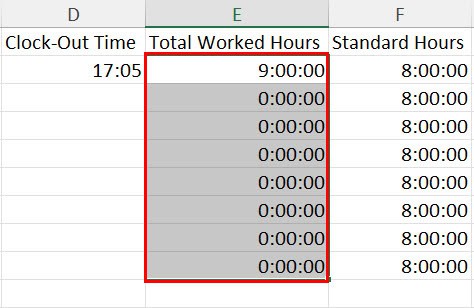
6. The calculated values of the Total Worked Hours column will now show as 9:00:00, 0:00:00, etc., which clearly indicates hours, minutes, and seconds.

7. To calculate overtime, enter the following formula into the first cell below the header of column G:

=IF(E2>F2,(E2-F2),(F2-E2))

8. Hit Enter to check if the formula is working.
9. Now, use the fill handle to copy the formula across the whole column.
10. Apply the [h]:mm:ss formatting code from the Format Cells dialog box.
11. Now, you’ll get overtime values in the HH:MM:SS format.

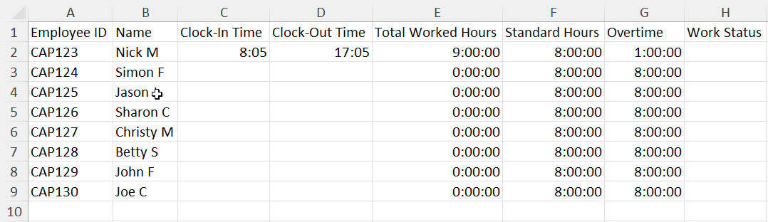
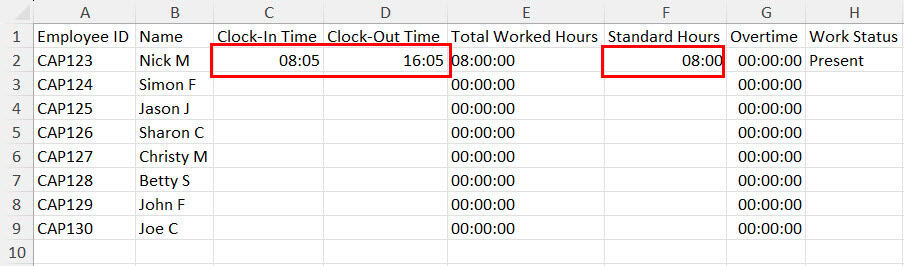
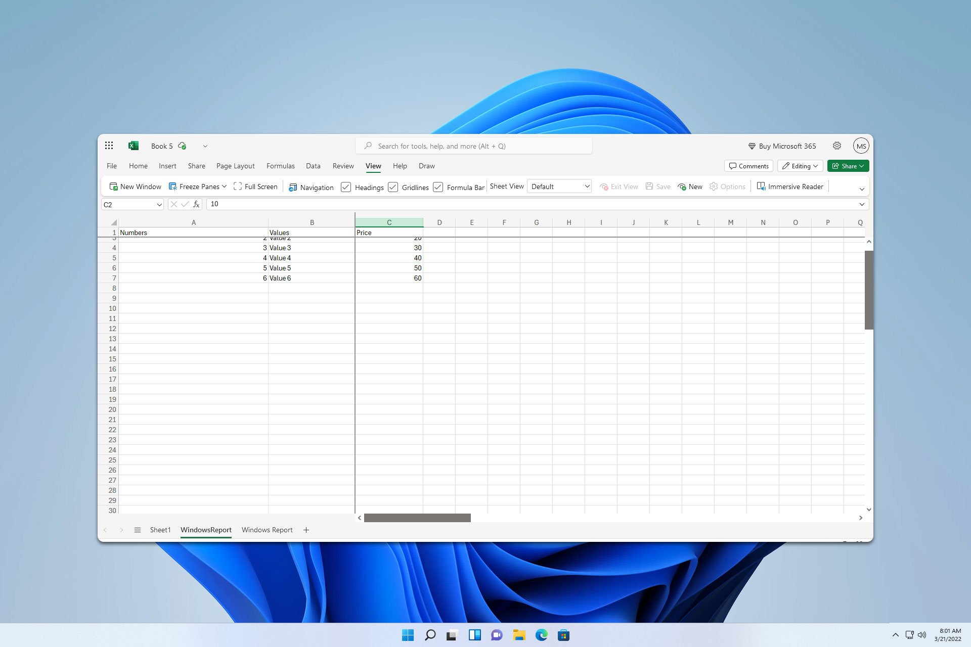
So far, the attendance sheet should look like the one shown below:

Replicate the Worksheet

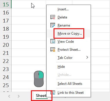
1. Right-click on the worksheet tab at the bottom.
2. Choose the Move or Copy option.

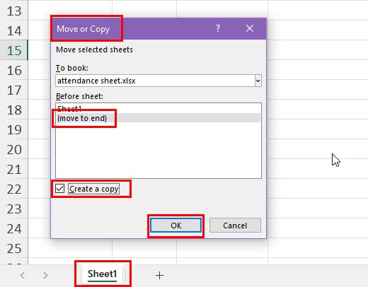
3. On the Move or Copy dialog, select the (move to end) option.
4. Checkmark the Create a copy checkbox.
5. Click OK.

6. This should create a copy of the existing worksheet.
7. Repeat the above steps to create copies when necessary.
8. Now, rename the first worksheet to the first date of the month.
9. You can create copies and rename those with the appropriate date for workdays.

Share the Worksheet With the Team

You’ve successfully created an attendance sheet in Excel.

For offline sharing, put the Excel workbook in a shared drive. Now, all the employees with access to the shared drive, can open and mark their attendance in the workbook.

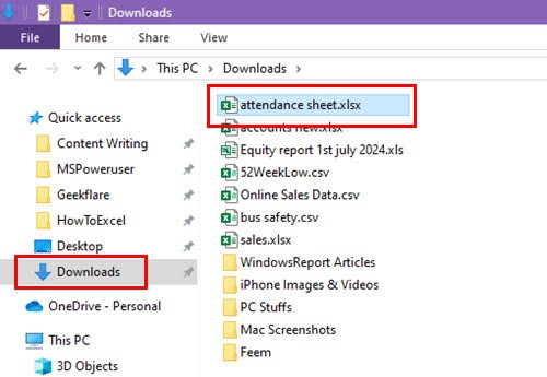
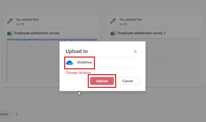
For online sharing, upload the Excel workbook to your OneDrive account.

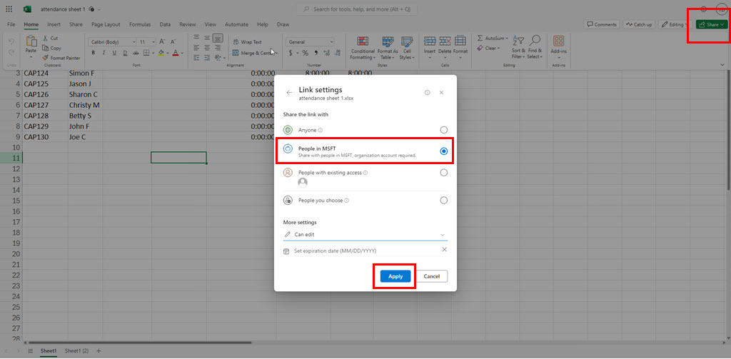
Create a shareable link for the document. Then, email the link to all employees who need to mark their attendance.

How To Make an Attendance Sheet in Excel Using Excel VBA

Find below a simple Excel VBA script to create an attendance sheet:

1. Open the target worksheet where you want the attendance sheet.
2. Press Alt + F11 to launch the Excel VBA tool.
3. Click the Insert button in the toolbar area and choose Module.

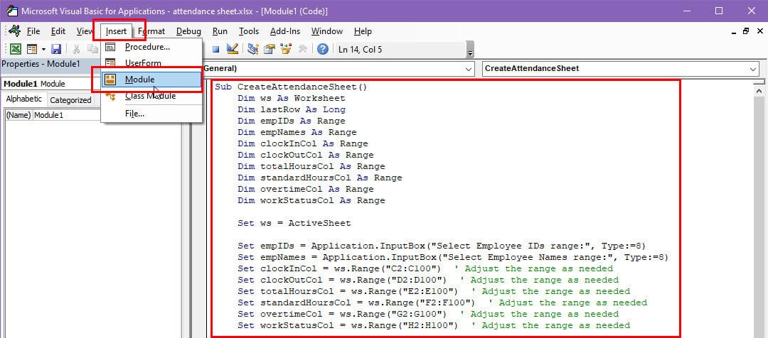
4. Into the blank module field, enter the following script:

Sub CreateAttendanceSheet()
    Dim ws As Worksheet
    Dim lastRow As Long
    Dim empIDs As Range
    Dim empNames As Range
    Dim clockInCol As Range
    Dim clockOutCol As Range
    Dim totalHoursCol As Range
    Dim standardHoursCol As Range
    Dim overtimeCol As Range
    Dim workStatusCol As Range
    
    Set ws = ActiveSheet
    
    Set empIDs = Application.InputBox("Select Employee IDs range:", Type:=8)
    Set empNames = Application.InputBox("Select Employee Names range:", Type:=8)
    Set clockInCol = ws.Range("C2:C100")  ' Adjust the range as needed
    Set clockOutCol = ws.Range("D2:D100")  ' Adjust the range as needed
    Set totalHoursCol = ws.Range("E2:E100")  ' Adjust the range as needed
    Set standardHoursCol = ws.Range("F2:F100")  ' Adjust the range as needed
    Set overtimeCol = ws.Range("G2:G100")  ' Adjust the range as needed
    Set workStatusCol = ws.Range("H2:H100")  ' Adjust the range as needed
    
    With workStatusCol.Validation
        .Delete
        .Add Type:=xlValidateList, AlertStyle:=xlValidAlertStop, Operator:= _
            xlBetween, Formula1:="Present,Absent,Planned Leave,Sick Leave,Casual Leave,Partial Hours"
        .IgnoreBlank = True
        .InCellDropdown = True
        .ShowInput = True
        .ShowError = True
    End With
    
    ws.Cells(1, 1).Value = "Employee ID"
    ws.Cells(1, 2).Value = "Name"
    ws.Cells(1, 3).Value = "Clock-In Time"
    ws.Cells(1, 4).Value = "Clock-Out Time"
    ws.Cells(1, 5).Value = "Total Worked Hours"
    ws.Cells(1, 6).Value = "Standard Hours"
    ws.Cells(1, 7).Value = "Overtime"
    ws.Cells(1, 8).Value = "Work Status"
    
    lastRow = empIDs.Rows.Count
    ws.Range("A2:A" & lastRow + 1).Value = empIDs.Value
    ws.Range("B2:B" & lastRow + 1).Value = empNames.Value
    
    ws.Range("E2:E" & lastRow + 1).Formula = "=TEXT(D2-C2, ""hh:mm:ss"")"
    ws.Range("G2:G" & lastRow + 1).Formula = "=IF(E2>F2, E2-F2, 0)"
    
    clockInCol.NumberFormat = "hh:mm"
    clockOutCol.NumberFormat = "hh:mm"
    overtimeCol.NumberFormat = "hh:mm:ss"  ' Add this line for HH:MM:SS format
    
    ws.Cells.EntireColumn.AutoFit
End Sub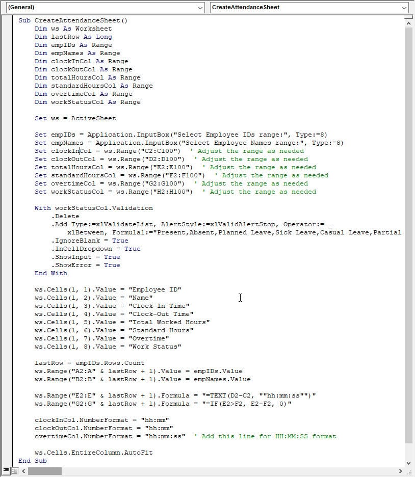

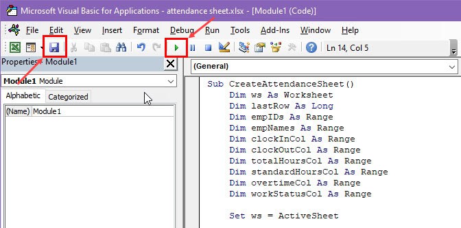
5. Click the Save button and choose Save in the dialog box that appears.
6. Hit the Run Sub button in the toolbar to execute the script.

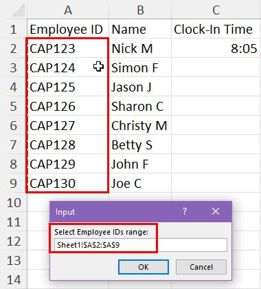
7. A dialog box will ask you to choose a cell range for employee IDs.

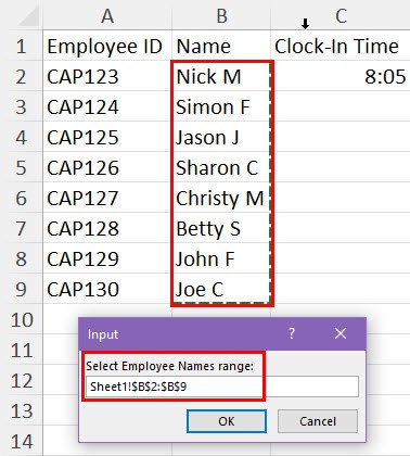
8. Similarly, select another cell range for the employee names.

9. Excel VBA will create the attendance sheet instantly.

Here are some tips on how to use this Excel attendance sheet effectively:

• Input any values between 00:00 and 23:59 in the Clock-In Time and Clock-Out Time columns.
• Enter the standard workday hour in the Standard Hours column in 08:00:00 format and copy the value across the column.

How To Make an Attendance Sheet in Excel With Templates

If you’re okay starting off from a ready-to-use template, I recommend these options:

1. Visit the Microsoft 365 Create portal.
2. Hover the mouse cursor over the Excel icon and click on the Browse templates button.

3. Enter the keyword Attendance sheet in the search box and hit Enter.
4. Choose one template from the results page.
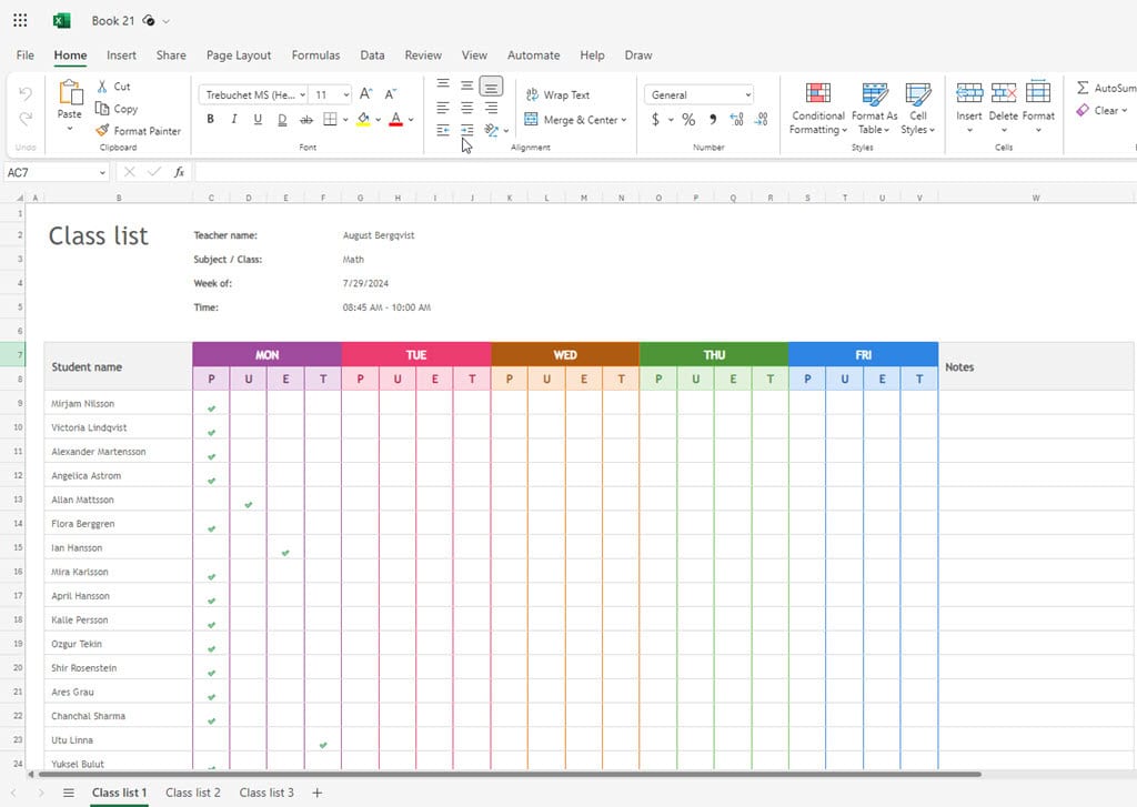
5. Click the Customize in Excel button.

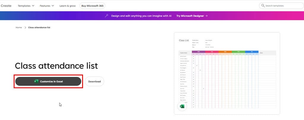
6. You should see a copy of the template in Excel online.

7. If you need an offline copy, click the Download button instead.

Summary

So, now you know how to make an attendance sheet in Excel in three different ways.

Comment below to let us know which method you like the most.

Additionally, if you wish to learn more Excel skills, you can check out unlocking grayed-out menus, resetting Excel to default settings, fixing #VALUE! error, and fixing Excel’s sharing violation error.