30 Excel Basic Formulas You Must Know

Excel is a popular spreadsheet software that offers a wide range of functionalities and is used by students, business professionals, or anyone who wants to organize information. Therefore, learning basic formulas is essential to enhance your data analysis and management skills. In this guide, we will mention 30 essential Excel formulas that you should know, ranging from operations like calculations, data manipulation, and logical operations.

What are the basic formulas you should know in Excel?

Basic Formulas: A Quick Overview

Formula	Syntax	Usage	Practical application
SUM	=SUM(number1, [number2], …)	Adds up the select range of numbers	Helpful in summing monthly expenses
AVERAGE	=AVERAGE(number1, [number2], …)	Calculates the average of a group of numbers	Used for determining the average score of a student
SUBTOTAL	=SUBTOTAL(function_num, ref1, …)	Calculates a subtotal in a list or database	Used for summarizing data in filtered lists
MIN	=MIN(number1, [number2], …)	Shows you the smallest number in a range.	Can be used to track the lowest temp over a month
MAX	=MAX(number1, [number2], …)	Shows you the largest number in a range.	Can be used to track the highest temp over a month
COUNT	=COUNT(value1, [value2], …)	Counts the number of cells that has numbers	Helpful in tracking the number of sales transactions in a month
COUNTA	=COUNTA(value1, [value2], …)	Counts the number of non-empty cells.	Allows you to keep track of completed tasks in a project
REPLACE	=REPLACE(old_text, start_num, num_chars, new_text)	Replaces part of a text string with another string.	Correcting a typo in the description of a product
SUBSTITUTE	=SUBSTITUTE(text, old_text, new_text, [instance_num])	Replacing occurrences of a specified text in a string.	Substituting the old term with a new term in large document
NOW	=NOW()	Displays current date and time	–
TODAY	=TODAY()	Shows the current date	You can calculate the number of days remaining before a project submission
TIME	=TIME(hour, minute, second)	Shows time in hour, minute, and second inputs.	Scheduling events by generating time stamps.
HOUR	=HOUR(serial_number)	Shows the hours from a time value.	Helping in extracting the hour from the timestamps
MINUTE	=MINUTE(serial_number)	Shows the minutes from a time value.	Can be used to check the time spent on various tasks.
SECOND	=SECOND(serial_number)	Shows the seconds from a time value.	Helpful in calculating the duration of video clips
MODULUS	=MOD(number, divisor)	Returns the remainder after division	Can be used to check if the number is odd or even
LEFT	=LEFT(text, [num_chars])	Shows you the specified number of characters from the start of a text string.	Helpful in extracting area codes from phone number
RIGHT	=RIGHT(text, [num_chars])	Shows you the specified number of characters from the end of a text string.	Can used to extract four digits of Social Security number
MID	=MID(text, start_num, num_chars)	Returns a specific number of characters from a text string, starting at a given position.	Used for extracting information from larger text
IF	=IF(logical_test, value_if_true, value_if_false)	Performs logical test and returns one value if TRUE and another if FALSE	Used to determine whether a student has failed or passed, depending on set threshold
DATEDIF	=DATEDIF(start_date, end_date, unit)	Calculates the difference between two dates in defined units	Helps in calculating age based on birthdate
POWER	=POWER(number, power)	Calculates a number raised to a specified power	Can be used for calculating compound interest
CEILING	=CEILING(number, significance)	Rounds a number up to the nearest specified multiple.	Helping in estimating project costs by rounding up to the nearest dollar
FLOOR	=FLOOR(number, significance)	Round a number down to the nearest specified multiple	Helping in adjusting values for budgeting and estimates
VLOOKUP	=VLOOKUP(lookup_value, table_array, col_index_num, [range_lookup])	Looks for a value in the first column of a table and returns a value from the same row in a specified column.	Searching prices for products on the basis of IDs
HLOOKUP	=HLOOKUP(lookup_value, table_array, row_index_num, [range_lookup])	Looks for a value in the first row of a table and returns a value from the same column in a specified row.	Fetching data from horizontal tables
TRIM	=TRIM(text)	Eliminates extra space from text, ensuring there is only single space between words	Useful for cleaning up the data entries
UPPER	=UPPER(text)	Changes text to uppercase	Writing names and codes properly
LOWER	=LOWER(text)	Changes text to lowercase	Writing emails addresses
PROPER	=PROPER(text)	Capitalizes the first letter of each word in a text string.	Helpful in formatting names in a list
CONCATENATE	=CONCATENATE(text1, [text2], …)	Combines multiple text strings into a single string	Used to merge first and last names into full name
LEN	=LEN(text)	Counts the total number of characters in a text string.	Used for checking the length of inputs in forms or data entries
INDEX-MATCH	=INDEX(array, MATCH(lookup_value, lookup_array, [match_type]))	Uses INDEX and MATCH together to search for values in a table more flexibly than VLOOKUP	Used in large datasets for more efficient data retrieval
COUNTIF	=COUNTIF(range, criteria)	Counts number of cells match a certain condition.	Helps you track the number of sales that go above a specific amount.
SUMIF	=SUMIF(range, criteria, [sum_range])	Sum values in a range that meets a certain condition	Used for calculating total sales of a product
IF-ELSE	=IF(condition, value_if_true, IF(condition2, value_if_true2, value_if_false))	IF statements to assess multiple conditions	Used for classifying performance ratings on the basis of multiple criteria
IFERROR	=IFERROR(value, value_if_error)	Returns a specified value if the formula shows an error, else returns the formula result.	Managing errors in calculations in data processing

If any of your Excel formulas disappear after you save your workbook, it could be because the formula is too complex and exceeds the memory capacity or is too long/complex; read this guide to learn more about it and the solutions to fix it.

1. SUM

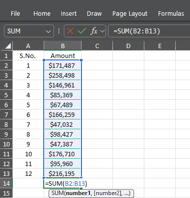
The SUM function is a basic Excel formula that can be used to add a series of numbers together. You can quickly calculate the totals from the selected range. For example, if you want to find the total sales from cells B2: B13 as in the picture, type = SUM(B2: B13) and press Enter.
This will add all the values within the selected range. The SUM function’s efficiency allows it to handle large datasets and simple totals, ensuring you can complete your numerical analysis quickly and accurately.

If the SUM formula doesn’t add the values correctly, it could be due to wrong cell references, hidden rows or columns, or cells with text or errors; read this guide to learn more.

2. AVERAGE

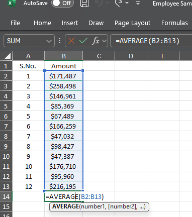
The AVERAGE function calculates the mean of selected numbers, giving insights into overall trends and is useful for measuring performance.

For example, if you want to find the average sales amount in cells B2: B13, use AVERAGE(B2: B13) and press Enter. This function adds up the values in the selected range and divides them by the count of numbers to calculate the average. This can be beneficial in financial forecasting and performance reviews.

3. SUBTOTAL

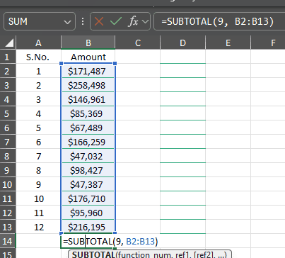
The SUBTOTAL function allows you to calculate aggregate values in a filtered database. It only calculates the relevant entries without including the excluded data. Unlike SUM functions, SUBTOTAL doesn’t include hidden rows, making it ideal for summarizing visible data.

For example, if you use =SUBTOTAL(9, B2: B13) and hit Enter, you will get the total of the visible values in that range. The number 9 in the formula represents the SUM function, so don’t change it. You can use it on pivot tables and filtered lists.

4. MIN and MAX

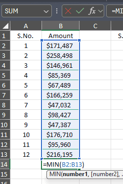
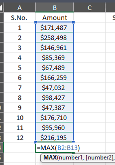
The MIN and MAX functions help you find the smallest and largest values in a selected range. For example, if you type =MIN(B2: B13) and hit Enter, it will show you the smallest value from the specified range. However, you will get the largest number if you type =MAX(B2: B13) and press Enter.

These functions are theoretical concepts and practical tools that you can use to identify extremes in your data. Whether it’s the lowest and highest sales figures, test scores, or any other data point, the MIN and MAX functions help you make sense of your data.

5. COUNT

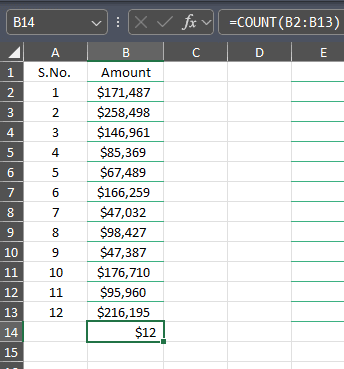
The COUNT function counts the number of cells containing numeric values within the selected range. For example, if you type =COUNT(B2: B13) and press Enter, you will get the number of cells in that range containing numbers.

This basic Excel formula can be helpful in statistical analysis, as it allows you to understand how many data points are numeric. It can also help you in data validation and ensure the datasets are complete, making data management easier.

6. COUNTA

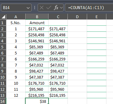
COUNTA is a formula that counts all non-empty cells in a selected area, regardless of whether they contain text, numbers, or errors.

For instance, the formula =COUNTA(A1:C13) will give you the number of cells with data in the area. This can help you track progress in datasets, such as counting completed tasks. Its efficiency in providing data usage insights surpasses COUNT’s, making it an essential tool in data analysis.

7. REPLACE

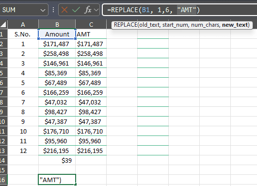
The REPLACE function allows you to change a portion of a text string based on chosen parameters. For example, if you type =REPLACE(B1, 1, 6, “AMT”) and press Enter, it will replace the first six characters in cell A1 with AMT starting with the first character.

This function allows you to correct errors or update specific text parts, such as typos. This is important for streamlining data management and enhancing efficiency in text processing.

8. SUBSTITUTE

SUBSTITUTE replaces specific occurrences of a text string within another string, which gives you precise control over text changes.

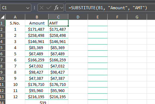
For instance, if you type =SUBSTITUTE(B1, “Amount”, “AMT”) and hit Enter, it will replace Amount with AMT in the text found in cell B1. You can use this formula to make changes in multiple places in a document. This basic formula of Excel can help change outdated terms, correct repeated errors, and ensure clarity in your data.

9. NOW

The NOW formula shows the current date and time, which can be helpful when time-stamping data entries or tracking changes.

To get the exact date and time, you must type =NOW() and hit Enter. This is a dynamic function, so the date and time are updated every time the spreadsheet recalculates. This can benefit project management, scheduling, and real-time event tracking.

10. TODAY

The TODAY function gives the current date without the exact time, which can be ideal for date-based timelines.

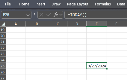
To get today’s date, type =TODAY() and press Enter. You can use this formula when setting deadlines and tracking time in projects.

The TODAY function is dynamic, meaning it automatically updates the date when the spreadsheet is opened. This feature is particularly useful for maintaining up-to-date reports, planning tools, and more.

11. TIME()

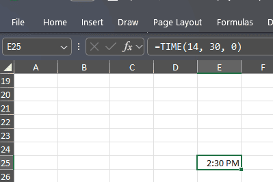
The TIME function shows you a time value in specified hour, minute, and second inputs.

For example, if you type TIME(14, 30, 0) and press Enter to execute it, you will get 2:30 PM as the output. You can use this function to schedule events and calculate time intervals in tasks.

This basic formula of Excel allows you to generate precise time values, which can be helpful time management, promoting better organization and planning

 12. HOUR, MINUTE, SECOND

HOUR, MINUTE, and SECOND functions retrieve hour, minute, or second from the time value selected. For example, if you type=HOUR(L1) and press Enter, this will extract the hour component from the time in cell L1. Similarly, if you type =MINUTE(L1) or =SECOND(L1) and press Enter, you can get the minutes and seconds mentioned in the cell.

You can use these basic Excel formulas while analyzing time and breaking down the time data for detailed reporting, including time spent on tasks.

13. MODULUS

The MODULUS function shows the remainder after division, which can be helpful for mathematical checks. For example, type =MOD(J1, 2) and press Enter, it determines whether the value in cell J1 is even or odd( it returns 0 for even).
This function can categorize data or implement periodic tasks. It can also simplify complex calculations, speed up processes, and facilitate batch processing.

14. LEFT, RIGHT, MID

The LEFT, RIGHT, and MID functions show you specific characters from text. Left will display the number of characters from the start. Type =LEFT(K1, 3) and press Enter, and you will get the first three characters.

However, if you type =RIGHT(K1, 4) and hit Enter, you will extract characters from the end. For MID, type =MID(K1, 2, 5) and press Enter to get the middle characters starting from the specified position.

You can also use these functions for data parsing, like extracting area codes from phone numbers.

15. IF

The IF formula allows you to perform a logical test and gives different values based on the result.

For example, if you type =IF(L1 >= 60, “Pass”, “Fail”) and hit Enter, it will evaluate whether the value in L1 meets the threshold of 60, so it will return “Pass” if true and “Fail” if false.

It is usually used for decision-making scenarios like performance evaluations and grading systems.

16. DATEDIF

DATEDIF calculates the difference between two dates in specified units: years, months, and days. For example, if you type =DATEDIF(M1, N1, “Y”) and press Enter, you will get the years between the dates mentioned in cells M1 and N1.
The DATEDIF function is a time-saving tool that automates date calculations. Whether calculating ages, tracking project durations, or simplifying date comparisons for planning and reporting, this function can handle it all, saving you time and effort.

Read more about this topic

• New Line in Cell in Excel: How to Start a New Row
• Microsoft Excel Keyboard Shortcuts: The Must Know List

17. POWER

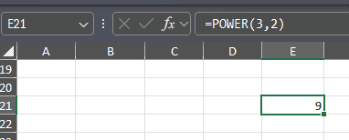
The POWER function raises a number to a certain power. For example, if you type =POWER(3, 2) and press Enter, you will get a result of 9.

This function enables you to perform complex calculations efficiently and is essential in financial projections and mathematical and scientific calculations.

18. CEILING

The CEILING function rounds up the number in a cell to the nearest specified multiple. For example, if you type =CEILING(O1, 10) and hit Enter, the value or number in cell O1 will be rounded off to the nearest ten.

You can use it in financial calculations, such as estimating budgets or costs, as it accurately rounds off values and provides a clear understanding.

19. VLOOKUP

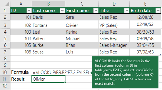
The VLOOKUP function looks for a value in the first column of a table and returns a related value from another column.

For example, if you type =VLOOKUP(B3, B2:E7,2, FALSE) and hit Enter, it will look for the value in B3 within the first column of the range B2:E7 and will show you the corresponding value from the second column.

YOu can use this function for data retrieval in large datasets, which makes accessing related information quickly, like prices or product details.

20. HLOOKUP

The HLOOKUP function works similarly to VLOOKUP, but it searches horizontally across the first row of a table. For example, if you type =HLOOKUP(Q1, A1:E5, 3, FALSE) and press Enter, it will find the value in Q1 in the first row and show you the corresponding value from the third row.

You can use it for horizontal tables like survey results or tabulated metrics, as it will help you retrieve data easily.

21. TRIM

The Trim function cleans up text by removing extra spaces from a string. It deleted leading spaces (spaces before the first character, trailing spaces (Spaces after the last character), and extra spaces between words.

For example, if cell A1 has the text ” Hello World “, you can type =TRIM(A1) and press Enter to get “Hello World”.

This function can be used if you are importing data from external sources, where there are spaces that can cause issues with data processing.

22. UPPER, LOWER, PROPER

The UPPER, LOWER, and PROPER are used to change the case of text in a cell. Upper changes the characters in a text string to uppercase. To do that, type =UPPER(R1) and hit Enter.

On the other hand, Lower changes all the characters to lowercase. To do that, type =LOWER(R1) and press Enter.

The Proper function capitalizes the first letter of each word. To do so, type =PROPER(R1) and hit Enter. You can use these functions to ensure the text in your data is uniform, enhancing readability.

23. FLOOR

The FLOOR function rounds a number down to the nearest specified multiple. For example, if you type =FLOOR(O1, 5) and press Enter, the value or number in cell O1 will be rounded off to the nearest five.

You can use this function in calculating discounts or at the time of budgeting. This function makes precise calculations, ensuring accuracy in financial reporting.

24. CONCATENATE

The CONCATENATE function allows you to join multiple text strings into a single string. For example, if you type =CONCATENATE(T1, ” “, U1) and hit Enter, it will combine the content of both T1 and U1 with a space in between.

This function is used in creating full names from first, middle and last names correctly. You can also use it to merge information from different cells into a single field.

25. LEN

The LEN function counts the number of characters, including spaces and punctuation, in a text string. For example, if you type =LEN(V1) and press Enter, you will get the character count of the text in V1 cell.

You can use this function for data entry, content creation and more as it can help validate input lengths in forms, and also helps manage text efficiently

 26. INDEX-MATCH

The INDEX-MATCH combo can improve data lookup capabilities and is considered an improved version of VLOOKUP.

INDEX displays the value of a cell in a selected row and column, while MATCH finds the value’s position within the selected range.

For example, if you type =INDEX(A1:A10, MATCH(W1, B1:B10, 0)) and hit Enter, it will search for the value mentioned in V1 within B1 to B10, returning to a matching value from A1 to A10. This combination formula makes handling large datasets easy.

27. COUNTIF

The COUNTIF function counts the number of cells if they meet a specific criterion within the selected range. For example, if you type =COUNTIF(X1:X10, “>100”) and press Enter, it will count the values in range X1 to X10 greater than 100.

You can use it to track sales above a target or count occurrences of specific conditions. It can provide important insights into datasets, which helps you make data-driven decisions wisely.

28. SUMIF

The SUMIF function adds up the values in cells under a specified condition within the selected range. For instance, if you type =SUMIF(Y1:Y10, “>100”, Z1:Z10) and hit Enter, it will add up the values in Z1 to Z10 that match with cells in Y1 to Y10 that are greater than 100.

You can use this function to calculate totals based on specific criteria and, therefore, be helpful in budgeting and reporting.

 29. If-Else

The If-Else function in Excel allows the application of conditional logic in formulas. It works like the IF function but comes with multiple other conditions.

For example, you can use =IF(A1 > 90, “Excellent”, IF(A1 > 75, “Good”, “Needs Improvement”)) to distinguish scores. This function can help you make complex decisions in data analysis and categorize data based on various scenarios.

30. If-Error

The IFERROR function allows you to capture and manage errors in formulas as it provides an alternate result when an error appears. For example, if you type =IFERROR(A1/B1, “Error in Calculation”) and press Enter, wherein A1 is 10 while B1 is 0, it will result in an Error in Calculation as you can’t divide a number by zero.

This formula can help you avoid confusing error messages and enhance the robustness of data analysis, thereby improving the overall user experience.

Conclusion

These are the basic Excel formulas you can use to transform the way you analyze your data. As you become familiar with these functions, you can gain deeper insights into your data and make better decisions.

If your Excel file is not opening when double-clicked it could be due to DDE settings; read this guide to learn other solutions. In case, you see the There’s a Problem With This Formula message in Excel, it could be due to syntax, or incorrect system settings; read this guide to learn more.

Which Excel basic formula do you use the most? Share it with our readers in the comments section below. We would love to interact with you.