Excel YEAR Function Not Working: 9 Best Fixes
8 min. read
Published on
Read our disclosure page to find out how can you help Windows Report sustain the editorial team. Read more
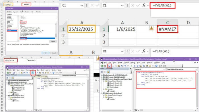
How can you fix the Excel YEAR function when it’s not working?
It’s one of the easiest ways to extract a year component from a long or short date in Microsoft Excel. However, this function is prone to many errors especially if the source data value isn’t in the right Date format.
So, I’ve recreated some Excel YEAR function issues that you may face. Here are the fixes that worked out for me the best!
How To Fix Excel YEAR Function Not Working
Before you start troubleshooting, ensure you’re using a supported Windows, Mac, or web app. The function is only available in Excel 2016 for Windows and Mac and newer, and the web version. If you’re using any earlier desktop editions, unfortunately, it won’t work.
Choose the Right Function Syntax
The most common mistake is not spelling the function syntax correctly. This causes the entire formula to break down. The Excel warning you get in this situation is the #NAME? error.
To avoid spelling issues, you must use the function suggestion as shown on the cell when you type initials after the equals sign.
You can scroll down or up to find the one you need and simply double-click to add it along with the opening parenthesis.
You can now type the rest of the formula arguments. Refer to the contextual suggestions for the valid arguments just below the cell where you’re typing to avoid flaws in argument construction.
Value Isn’t in the Date Format
Here are the possible slip-ups you might make while using the YEAR function:
- Non-date text values: When the input argument is a text string that Excel can’t recognize as a valid date, you’ll see an error.
- Blank cells treated as text: If Excel treats a blank cell as a text string, the function will show the #VALUE! error.
- Date in an invalid format: If you use an unsupported date format, like “21/06/2025,” you’ll get the #VALUE! error.
- Logical values or arrays: This mistake can happen mostly when the input cell reference of the YEAR function is derived from other Excel basic formulas. If the input is an array that doesn’t contain supported date values or these are logical values, like TRUE or FALSE, you’ll see an error.
- Non-numeric date values: If you use two thousand twenty-five instead of 2025 as an input, Excel will show the #VALUE! error.
- The cell contains an error: In this case, the YEAR function shows the #VALUE! error.
For example, this function has broken down because there’s a tilde sign in the referenced cell.
When I remove the accent sign, it works just fine.
Custom Date Formats
Another pressing problem with YEAR is its inability to appropriately detect the year value from a custom-formatted date. For example, it’ll work with popular date conventions, like YYYY/MM/DD or MM/DD/YYYY.
However, when you place the function with a DD/MM/YYYY or YYYY/DD/MM format, it fails to isolate the year.


Another way to get the same error is by using the Custom formatting category from the Format Cells dialog box.
If you select a cell and press the Ctrl + 1 keys, the Format Cells dialog box will show up. Now, go to Custom and enter any of the following date formats in the Type field:
- yy/dd/mm
- yy/mm/dd
If you now type any date in the custom-formatted cell, you’ll get an error for the YEAR function.
So, avoid the above custom date formatting instances.
Date Entries Formatted as Numbers
When you convert a date entry to the Number formatting style, the YEAR function shows an error.
Look at the screenshot below. When it’s in its correct form, like the Date format, the function can properly extract the year in cell C1.
However, changing the date to a Number format shows the #REF! error message.
Another scenario when you might experience the same issue is deleting the old entry and typing in a new value.
When you delete the previous entry in A1, Excel hard codes the YEAR function in the following syntax:
=YEAR(#REF!)
Now, if you update the referenced cell with a new value, Excel can’t detect that because it has automatically added the #REF! error to the YEAR function by replacing A1, which was the blank cell.
You can fix this issue by editing the arguments again. For example, replace #REF! in the formula syntax with A1.
The YEAR function will calculate the year value again.
Hidden Characters or Spaces
Hidden characters, like non-breaking spaces, change the appropriate formatting of date entries. When you refer your YEAR function to any such cells, you’ll get a #VALUE! error.
To clear these unwanted characters from your dataset, press Alt + F11 to launch Excel VBA Editor.
Right-click on the current workbook in the left-side navigation panel of the VBA Editor. Hover the cursor over Insert and select Module from the context menu.
A blank module will open on the right.
There, copy and paste the following VBA script:
Sub ClearHiddenCharacters()
    Dim cell As Range
    For Each cell In Selection
        cell.Value = Replace(cell.Value, ChrW(8203), "")
        cell.Value = Replace(cell.Value, Chr(160), "")
    Next cell
End Sub
Hit the Save button on the toolbar.
Now, select the worksheet dataset from which you wish to remove hidden characters.
Click on the Run button on the toolbar or hit F5 on the keyboard.
Excel VBA macro will clean the dataset automatically.
The YEAR function also instantly calculates the cell and shows the year value.
Dates Beyond Excel’s Supported Range
The YEAR function is only effective within a year range of 1900 and 9999. If you refer to an input cell containing a year below or above the given range, the function will either show an error message or an incorrect value.
For example, I entered 01/01/1899 in A1 and used the =YEAR(A1) syntax in C1.
I got the #VALUE! error.
The same error will show up when the input date is 01/01/10000.
So, check if the input has a year value outside the given range to fix the issue.
Regional Settings Mismatch
If the region settings in the PC and Microsoft 365 Admin Center don’t match, Excel might process date formats incorrectly.
First, ensure your PC is set to the desired region configuration by clicking the ENG icon in the System tray.
English (United States) should be on the top of any other input languages if you’re in the US or following the US input format.
If you don’t see the US option, click on the Language preferences option.
Click on the Add a language button below the Preferred languages section.
Find and select English (United States). Click Next.
Now, navigate to your Microsoft 365 Admin Center portal.
Type Region in the top search field and select My settings and privacy.
You’ll now arrive on the Settings & Privacy page. Navigate to the Language & Region tab on the right.
Now, click on the Region format option and select Change regional format button.
Select the English (United States) format from the list.
You’ll see a sample date confirming that you’ve successfully selected English (United States) as the region.
Now, restart the Excel desktop app.
Try using the YEAR function and this time it should be able to extract the year from the date.
Negative or Non-Gregorian Dates
The YEAR function works well with Gregorian calendar dates. Even if you refer to a non-Gregorian calendar date, it’ll try to show the equivalent year.
For example, the following screenshot shows that the argument is referencing cell A1 which has a date from the Hijri calendar. Therefore, the function can’t extract the year value appropriately and shows the #VALUE! error.
Moreover, if the input date value comes with a minus sign, the YEAR function won’t be able to calculate the year entry because Excel converts the source data into a negative fraction.
So, ensure there are no negative dates in the input dataset.
Use YEARFRAC for Fractional Year Values
If you’re trying to extract the number of years from a start and end date, you’ll get an incorrect result with the YEAR function.
It’ll process it as an input value and derive the corresponding year if possible, but not the actual calculated value.
For instance, if you subtract the end date 12/10/2024 from the start date 6/10/2025 in Excel, it returns 1643. Now, the YEAR function converts 1643 to 1904 instead of 4.5 years.
Here, you can use the following formula with the YEARFRAC function to quickly get the calculated year.
=YEARFRAC(A2,B2)In the above formula, A2 is the start date and B2 is the end date.
Excel will calculate and extract the number of years elapsed, which is 4.5.
Summary
Now you know what to do when the Excel YEAR function is not working.
Did any of the above methods work for you? Do you know of a better approach? Share your thoughts below.





User forum
0 messages